When I say temperature sensors, you’ll likely think thermocouples. But today I’d like to discuss NTC thermistors. Medical devices regularly need to measure  temperature. Often engineers overlook or under-estimate the inherent challenges. Whether designing in thermal measurement and control capability or just temporarily instrumenting up a test rig, it’s worth thinking about how the device measurement is going to work.

The fundamental concept is to stick a temperature sensor in a place on the device where heat will be exchanged with the item whose temperature we wish to measure. Challenges arise when that path is not sufficiently dominant over parasitic paths to other sources of heat. For example, measuring gas temperatures is particularly challenging; often the wire leads of the sensors carry more heat than expected to be exchanged with the gas. In addition, combining these thermal resistances with the thermal masses of the various path elements can result in a system that is too slow to measure interesting transients.

These are temperature dependent resistors and they come in two general varieties: positive temperature coefficients (PTC) and negative temperature coefficients (NTC). Although PTC devices are useful for many applications, I’m going to limit this conversation to the NTC variety.

NTC thermistors are relatively inexpensive devices and come in many shapes and sizes, from small printed circuit board (PCB) mounted devices, to glass-encapsulated beds with wire leads. Unlike thermocouples, they don’t need a cold junction, and their large change in resistance make them fairly noise immune without the need for amplification. On the down-side, their temperature-resistance relationship is annoyingly non-linear.

Temperature vs Resistance

NTC thermistors are accurately approximated by the Steinhart-Hart (S-H) equation. At first, this seems mathematically ugly but once you get over the natural log and the inverse relationship with absolute temperature, it’s really just a third order polynomial.

Note that the traditional equation form does not include a quadratic term. I have found that adding one often improves the overall accuracy.

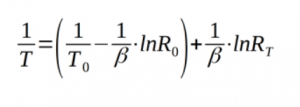
A slightly simpler option is the thermistor beta equation. This is just a special case of the S-H equation where the quadratic and cubic terms are removed.  The advantage of this equation is that you can get reasonable computed accuracy with only two parameters. The nominal values of these are often quoted on thermistor datasheets.

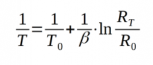
Here’s the same equation again but expressed in a form that easily compares to S-H.

Typical Circuit
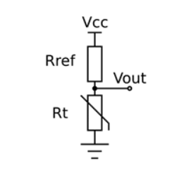
A typical NTC thermistor circuit implementation is simply a resistor divider formed with the thermistor and a reference resistor. The reference resistor is usually chosen to be equal to the thermistor resistance at a temperature point within the range of interest. Often 25 C is used, as the resistance at that temperature is usually a specified parameter of common thermistors.

This circuit not awesomely linear, but by choosing the reference resistor carefully, it can be good enough as it is for many applications. Note that the reference resistor is just as important to the stability and repeatability of the circuit as the thermistor. We have to watch out for the resistor’s initial tolerance as well as its temperature coefficient.

Variations to this circuit include adding a filter capacitor to roll-off high frequency noise and swapping the thermistor and resistor, thereby creating a voltage that increases with temperature instead.

In many applications this divider is sampled directly by an Analog to Digital Conversion (ADC) to achieve a ratiometric measurement for further computation in firmware. The divider output can also be fed directly into downstream circuits for feedback control systems or interlocks.

Linearization

An initial concern with NTC thermistors is the non-linear response. Converting the voltage output of the divider circuit to an accurate temperature measurement is often perceived as tricky.

Here are a few strategies that I have used successfully in the order of increasing complexity:

• Single Point Measurement

For many applications, we’re only interested in a single temperature. For these situations, the reference resistor can be chosen to achieve a desired threshold voltage at that temperature. In many cases that’s all we need. Sometimes the threshold can be implemented in firmware either as a hard-coded value to achieve nominal accuracy or as a calibrated value for the highest accuracy at that single point.

• Linear approximation

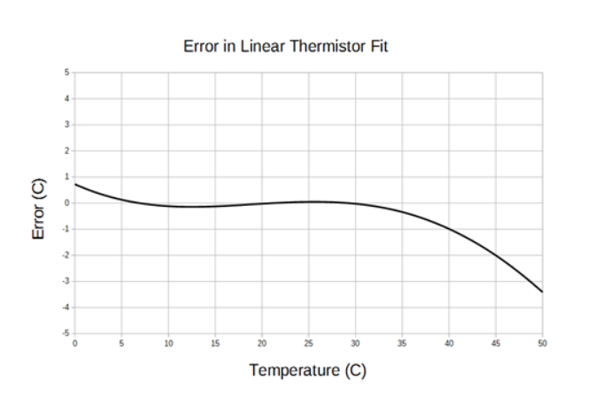
If accuracy is not a primary concern, then a linear approximation of the divider output may be sufficient. By choosing the reference resistor carefully, a limited temperature range can be defined with pretty low error, but the error will increase steadily outside of that range. This is often acceptable: it gives good accuracy around a point of interest, but still gives an idea of how far away from that point the present reading is.

The following graph shows an example of temperature sensing error when using a simple linear fit of the divider voltage, optimized for 25 Celsius. The fit is really pretty good between 20 C and 30 C.

• Interpolated Lookup Table

A common approach to achieve good accuracy when linearizing NTC thermistors is simply to program in the resistance vs temperature lookup table (LUT) specified by the manufacturer. This can be used with as much resolution as desired and then further resolution can be achieved with linear interpolation between the points. A good strategy is to implement the LUT as ADC value vs Temperature. This is computationally simple, but it assumes that the application is ok with the natural variation that occurs from part to part. If part tolerance leads to unacceptable accuracy, then individual calibration will be required and an LUT is no longer a good choice.

• Beta

A next level of accuracy can be achieved by implementing the thermistor beta equation. As a rule, this can get you below half a degree Kelvin within a reasonable range of temperature. By computing a custom beta value, you can choose where the accuracy is optimized. Typically, this beta value will be custom computed from real calibration data, although using the datasheet (i.e. nominal) value may still yield sufficient accuracy for many applications. If your microcontroller has a math coprocessor then this can still be quick enough to compute. Consider an LUT to get from ADC reading to the log value as a hybrid solution.

• Full Steinhart-Hart

A final jump in accuracy – especially over a wide range of temperature – can be achieved by a full-blown implementation of the S-H equation. Usually this goes hand in hand with the need to perform a multi-point calibration, but I have used this approach in the past to generate an LUT during initialization instead of copying a big data table into my source code.

A variation of the S-H equation that I prefer is to use the log of the ratio of thermistor resistance to the reference resistor value, instead of just the log of thermistor resistance. This is convenient because I can easily compute that from my ADC value. In this situation it’s best to include all four terms.

Calibration

As I’ve mentioned, to get that final jump in accuracy, some amount of calibration will be required. The linearization strategy employed will determine how many temperature points will be required.

Fundamentally, calibration consists of applying a known temperature and then adjusting circuit or software parameters based on the measured response. Applying a known temperature is a two-step process. First, we apply a calibrated sensor to our system, and then we control the temperature of our system until the calibrated sensor reads the desired value. Once the value has been achieved, we check the state of the sensor we’re trying to calibrate. We repeat that process for as many temperature points as we need. The calibrated sensor could be a jig made with another thermistor that we’ve sent to a National Institute of Standards and Technology (NIST)-traceable lab for measurement over our range of interest, or a PT100 style PTC thermistor that also has been NIST calibrated.

One example of a calibration setup involves temporarily applying a calibrated sensor to our device and causing the device to change its own temperature. Another example is to apply a calibrated sensor to a stirred water bath and insert part, or all, of our device into the bath.

During calibration we also need to think through desired and parasitic sources of heat and their associated thermal path resistances. No matter how awesome we believe our calibrated sensor to be, it won’t yield good results if we can’t make it reliably equilibrate with the right part of our device. Also, for each calibration point, we must allow enough time for all the thermal elements to reach their final temperature. Depending on the thermal masses involved, this might take many minutes or possibly much longer.

If single point accuracy is all that is required – because we’re just using a threshold in our device – then a single calibration measurement at that point is all that is required.

If we’re using the beta approach, then a minimum of two points is required. To compute beta, a linear regression between inverse-temperature and the natural log of resistance-ratio is a good method. This will yield an offset-term coefficient and a linear-term coefficient. The inverse of the linear-term coefficient is our new beta value.

To calibrate for the full S-H equation is not so different from a beta calibration, but more points will be required within the range of interest. Running through a multi-point calibration is usually done with an automated test setup. For that reason, I like to use around ten points. A four parameter least-squares regression is a good way to compute the S-H parameters.

One important thing to remember, if you are computing calibration parameters, is that you may need to do a final QC temperature-sweep to check that the system is measuring within the required accuracy after calibration.