This blog builds upon a great post by Mark Drlik. Mark focused on a specific application of the technique introduced by Stuart Pugh in his masterpiece “Concept Selection – A Method that Works.” We’ll take a step back and revisit Kepner-Tregoe’s original Decision Matrix, then propose tweaks to make it broader and more robust.

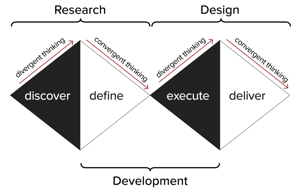
Let’s use an example that illustrates the Decision Matrix method by using it along with the Double Diamond design framework to create and select candidate solutions. The Double Diamond framework has four phases as shown in the image at the top of this blog. Those phases have been phrased in different ways along the years and across industries. I’ll be using:

1. discover (divergent thinking)
2. define (convergent thinking)
3. execute (divergent thinking)
4. deliver (convergent thinking).

Note that the terms divergent thinking and convergent thinking are a Design notation. This article also uses the terms grafting and pruning, respectively. The latter pair is an analogy borrowed from the Decision Making field, which seems appropriate since this work deals with Decision Making applied to the Design Process. The Decision Makers use a tree analogy: ideas are branches that are grafted and then pruned while goals (i.e., prototypes or end products) are leaves.

The four design phases above are divided into two sub phases:

1. the first sub phase is grafting and pruning candidate solutions (discovering and then defining them, i.e., using divergent and then convergent thinking);
2. the second sub phase is a more mature round of divergent and then convergent thinking, i.e., grafting and then pruning candidate solutions (executing and delivering them, respectively).

During the first phase of the Double Diamond (discover candidate solutions), the process is to brainstorm and graft twelve possible solutions. Now it’s prune time (define candidate solutions). The goal of this step is to reduce the twelve solutions down to three solutions which will be developed further using StarFish Phase Zero prototyping processes (i.e., sketching and then creating physical models of the concepts). How to narrow down from those twelve to the three more promising concepts?  By using a weighted decision matrix method as presented below.

Note 1: The criteria for the prototype design exercise are Mass, Cost, Robustness, Manufacturability, Electrical power usage, and Hazardous emissions.

Note 2: For the sake of readability and concept flow, I only show four candidate solutions, not all twelve.

Note 3: What happens after the process that this blog post describes: I proceed to the second graft-then-prune pass (i.e., execute and then deliver) in the second diamond of the Double Diamond method. That second diamond narrows three solutions down to one, which will be further developed. This will not be covered by the article.

Table 1: A Weighted Decision Matrix in its simplest form.

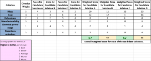
The Weighted Decision Matrix Process in its simplest* form is manifested in the table above, and is created by following the steps below.

1) Create a criteria to rank your candidate solutions, e.g. cost, manufacturability, electrical power usage, hazardous emissions, mass (Table 1, “Criterion” column).
2) Choose a weight (importance) for each of the criteria (Table 1, “Criterion Weight” column): I’ll use numbers from 1 to 5. Note that “higher is more important”. Hence, if cost is highly important to you, choose 4 or 5. If electrical power usage is of little importance, choose, 1 or 2. This way, if you want to rethink the weighting of the criterion later, all you have to do is change the weight to a different number between zero and 5.
3) For each of the candidate solutions, assign a score for each of the criteria: if the candidate solution A ranks average for hazardous emissions, use 3. If candidate solution B is efficient with electrical energy, you might want to use 4 (Table 1, “Score for Candidate Solution” columns).
4) Each score has to be adjusted by its importance. Hence, multiply it by the criterion weight. Now I have weighted scores for each cell, which represents how well a candidate solution scores according to a criterion – taking into account how important the criterion is (Table 1, “Weighted Score for Candidate Solution” columns).
5) For each candidate solution, add all the adjusted scores (from the first to the last criterion), and you’ll have the overall weighted score for that solution. This is shown at the bottom of the table: the weighted scores are 57, 50, 57, and 56 for candidate solutions A, B, C, and D, respectively.
6) Hence, candidate solutions A and C tie as the best ones according to this set of criteria, criteria weighting, and scoring per candidate solution per criterion. Candidate solution B, on the other hand, is deemed the least desirable one.

* You might argue that if the matrix was not weighted, it would be even simpler, but I will be using weighted evaluation functions as a premise. In case you’re wondering, an evaluation function is a mathematical model which describes how good a candidate solution is. It’s the foundation of many decision-making (and optimization) techniques. The overall weighted score above plays precisely that role.
I’ll now present some tweaks to improve the basic version of the technique presented above. But why do we need improvements in the first place? I’ll address one by one the weaknesses of the simplest version of the Decision Matrix and then explain how the tweaks will tackle those flaws.

Weaknesses of the simplest Decision matrix:

I. Sometimes you do not want to use the scores for all criteria as numbers from 1 to 5. That is especially true when using quantitative, eliminatory criteria e.g. mass. We’ll talk about eliminatory criteria on tweak III below. Tweak I will tackle this weakness.
II. A weighted arithmetic evaluation function might be too complacent with candidate solutions that rank very well on some criteria but too poorly on others. Tweak II will tackle this weakness.
III. Having all criteria as ranking-only might cause the design team to sketch and even physically prototype a solution that is hopeless (since there is no threshold for elimination). That is possible if that solution ranks very well in many criteria despite the fact that it is unsatisfactory according to one or more. Tweak III will tackle this weakness.
IV. Depending on if you use tweak I or not, you might have final outputs from the matrix (i.e., one overall weighted score per candidate solution) of different magnitudes. It would be ideal if across the organization, ranges would be always the same so that different studies, teams, and departments could speak the same language. Tweak IV will tackle this weakness.

Tweaks:

I. Use ratios (standardized grades) in the raw scores (i.e., the scores you choose, the inputs).
II. Use a weighted geometric evaluation function (instead of the weighted arithmetic one shown above).
III. Split the criteria into eliminatory and non-eliminatory criteria (the first requires definition of thresholds for elimination).
IV. After the overall weighted scores are done, turn them into ratios (i.e., standardized grades, e.g. from 0 to +1 or -1 to +1).

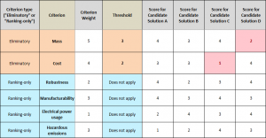
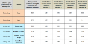
Table 2 shows the implementation of all the above tweaks. We’ll use it to elaborate on tweaks I and III, which are less self-explanatory.

Table 2: Implementation of the four tweaks for the Decision Matrix.

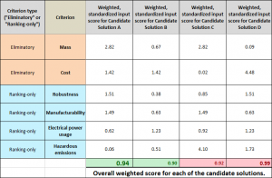
Tweak I
We’ll be starting from tweak I. As mentioned above, the technique is more robust if you standardize all your input scores. Hence, what we called step 3 in the process shown above will now be called 3.A. Also, steps 3.B and 3.C are now added. The result follows:

3.A) For each of the candidate solutions, assign a score to each of the criteria. Again, let’s use numbers from 1 to 5. Reminder that we’re still using “higher is better”.
3.B) For each criterion, we’ll be calculation a standard value. One option is to calculate the simple arithmetic mean of the scores for all the candidate solutions for that criterion (Table 2, “Average score (arithmetic mean) for criterion across candidate solutions” column). You can also use, as standard value, the absolute value of the score whose modulus is the highest, or the maximum possible score for that criterion (i.e., 5 if you are using scores from 1 to 5). The latter is especially useful when your goal is to create your range of possible outcomes such as the perfect solutions is – by definition – 1.00. Alternatively, you can use a baseline value. This is especially useful when you’re trying to improve an existing solution, as we many times do in the field of Engineering.
3.C) The standardized score is the raw score you entered divided by the arithmetic mean (or the score whose modulus is the highest, or the maximum possible score for that criterion, or the baseline value). That is shown in Table 2, “Standardized input score for Candidate Solution” columns.

Tweak III
As for tweak III, let’s say that one of the product requirements states a maximum permissible mass. We then chose to make mass an eliminatory criterion. Hence, we flag it as such (Table 2, “Criterion type (‘Eliminatory’ or ‘Ranking-only’)” column). Every eliminatory criterion requires a threshold which will either accept or reject each candidate solution based on its score for that criterion. The threshold connected to the mass criterion is shown in Table 2, “Threshold” column, as “3”.

If a candidate solution has a score that is worse than the threshold for that criterion (in the example, that means that it scores lower than 3 for mass), it will be rejected (Table 2, “Eliminated or Approved” columns), no matter how well that solution might have scored in the other criteria. That criterion can also be used to rank solutions, just like the non-eliminatory criteria**. It’s your choice. In this example, we chose to do so.

** Also known as “ranking-only criteria”, i.e., the non-eliminatory criteria are not associated with thresholds. That means that non-eliminatory criteria serve for ranking purposes but not for eliminatory purposes per se.

Results Discussion
As a result of this exercise, we have:

• rejected candidate solution D due to its mass (Table 2, “Eliminated or Approved (Candidate Solution D)” column). If that was not the case, that would be chosen as the best solution, since it has the highest overall weighted score (0.99).
• rejected candidate solution C due to its cost (Table 2, “Eliminated or Approved (Candidate Solution C)” column ).
• ranked the non-eliminated candidate solutions A and B as the best and the second-best, respectively, based on their overall weighted scores (0.94 and 0.90, respectively).

Note that given the way we chose the criteria weights (higher means more important) and scores (higher means better), the higher the overall weighted score, the better the solution. Also note that candidate solution A (score 0.94) was chosen over D (score 0.99) due to the fact that the latter was rejected by the eliminatory criterion “Mass”. That alone shows a great impact of Tweak III.