Anyone who has taken a signals and communications course has likely heard of matched filters. Intuitively these filters use knowledge of the form of a transmitted signal to pull it out of the noise. Matched filter theory or related concepts are commonly used in RF communication but I often apply it to other signals, such as sensor measurements in medical devices.

You may be familiar with chopping in optical systems or IQ detection in ultrasound imaging. These are applications of the principles of matched filters. Whatever the application, the goal is to make the highest accuracy signal measurement in the presence of spurious sources of error and noise.

Let’s consider the specific example of sensor measurement. Typically we inject some power into a system and measure the response in some way. For instance, to make a potentiostat measurement we set a voltage and measure a current. To make an optical density measurement we control the power output of an LED or laser source and measure a photosensor current that represents the light that has transmitted through our optical system.

Let’s assume that we have some ability to modulate the power input, either in an on-off or continuously variable fashion. Let’s also assume that the input and output values are always positive values. This is never the case for RF demodulation but must be for optical intensity and is often true with other sensor measurements as well. I’m going to make yet another assumption: that we’re solely in the digital, discrete time domain. In other words, I’m assuming I’m controlling the system input digitally with a DAC or maybe a simple enable signal, and reading back the sensor value with an ADC. I’m also going to make the assumption that the system is linear.

Intuitively the parameter that I would like to measure is the system gain. I want to know how much the output of the system changes for a given input change. There is also likely an offset associated with the input to output relationship as well, but typically this has little use. If I use the word “slope” instead of “gain”, I hope you’ll not be put off by my intuitive leap to computing a linear regression between input and output. To do this I vary the input and make a bunch of output measurements. The more measurements I make the better estimate of slope I get. Typically, if I was simply doing a regression I would vary the input in a series of increasing steps, until I had my desired sample size and then compute the slope and offset. The fact is, I don’t need to make the measurements in this order. I can set the input to any values, in any order I choose, so long as I end up with the desired number of measurements over the desired range of input values.

Now I’m going to get a bit mathy. Feel free to jump ahead to the punchline if you need some instant gratification.

To start with, let’s remember the good old equation that we’re trying to solve.

The input of our system is x, the output is y, the slope is m and the offset is b. Let’s assume for now that we want to use n samples to compute the slope and n is greater than 2. To get our bearings, let me put down the matrix form of the equation we’re trying to solve.

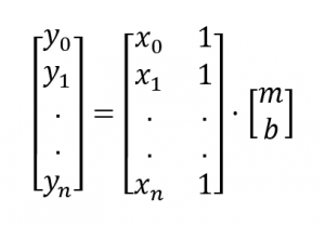
I can express this as a product of a matrix and vector to get the equation we want to solve.

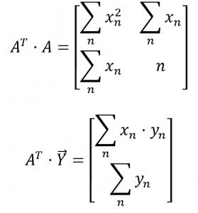
The matrix A is not square and therefore cannot simply be inverted. Instead we use a least squares approach to solving this system. I’ll just write down the matrix form of the least squares solution. It’s fun to derive if you have a minute or two but for now let’s skip to the final form.

So, let’s start digging into some of these terms.

And

To make these series of sums more attractive, I can write them in terms of summations.

Now let’s figure out some more terms.

Now we jam all these terms together to get to the solution of the original equation.

I’ll rearrange this a tad.

Here’s how we calculate the determinant.

I’ll rearrange this also.

You may notice that this equation is pretty similar to the equation for standard deviation. In fact, I can write it in the following way.

Another thing to notice is that there are a number of terms that look like the mean of various signals. For instance

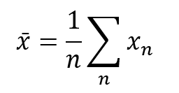
I’ve pointed out these identities because the input signal is something that we control and ideally we choose it to be periodic and repeating. This means we don’t need to compute a bunch of these summations all the time. Instead we can compute these values ahead of time and simply apply them as constants.

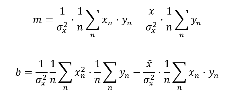
As you’ll recall, the first term of is the slope, and the second is the offset. Let me write them out explicitly after applying my identities.

You’ll notice that to compute the slope, I only need to keep track of two sums. I’ve also chosen to write these out in such a way that it’s clear that I’m really just computing averages. I need the average of the product of the input and output and I need the average of the output.

Getting down to practicalities, I can implement these averages in a number of different ways. I can use a rolling buffer and compute the slope each time I rotate in a new sample. I can accumulates n samples and only publish a new slope value every n^th sample. If I don’t have a ton of memory or processor horsepower and I want a long time constant, I can approximate these averages using single-pole, low-pass, IIR filters.

I’ll note at this point that for any AC-coupled signal the average output will be zero and therefore the second term disappears. All that remains is the integral of the product of input and output. The equation then starts to seem spookily familiar: the math it’s performing is exactly the same as the mixer in an IQ demodulator or in a synchronous detector. The input is really the carrier that I’m modulating my system with.

So, here’s the punchline as we finally come back to the magic of matched filters. If I choose the modulation well, then I can maximize my ability to select the actual signal I want and discriminate against noise and other sources of error. Some examples of typical sources of error are: AC line voltage coupled electrically or optically; RF or electromagnetic interference; thermal noise or drift and any other time varying signals in our system. If I choose my modulation to differ from the error sources then likely only the good stuff will survive its travels through the slope calculation. DC is rejected – it ends up in the offset – and in fact any noise that does not correlate with the modulation is also squashed. Don’t take my word for it; push whatever you like through that slope equation. You’ll see what I mean.

Here’s another cool trick. If I have more than one measurement to make with the same detector and different inputs, then I can modulate each input with signals that are orthogonal to each other. In other words, if I modulate with one, the other doesn’t get though the slope equation. The reverse will also be true. This can be achieved in a number of ways: different frequency sinusoidal carriers, orthogonal coding schemes, sine and cosine, or even time division multiplexing for that matter. This way I can happily measure many signals at once.

I hope I’ve given a slightly different take on matched filters compared to what you might have seen in university. You might even be inspired to look back through your old textbooks with a different perspective. Mind you, I won’t judge you if you don’t.