Lord Rutherford famously said “If your experiment needs statistics, you ought to have done a better experiment”.

In reality, when developing In-vitro Diagnostic Devices, and diagnostic devices in general, an algorithm is almost always required to convert the stream of electronic sensor data into a clinical relevant parameter – displaying volts or ADC counts is not usually sufficient.

Here are some helpful techniques for developing your next IVD algorithm:

Assessing Disease Discrimination Performance

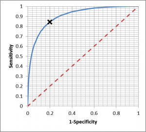
Previously, I discussed tests which give a quantitative index or yes/no answer.  Many tests provide a quantitative index which must be then converted to a binary decision, which requires a threshold to be defined – the so called “operating point”.  A very useful tool for evaluating operating point is the Receiver Operating Characteristic (ROC) curve –  first developed during world war two for the analysis of radar signals, hence the name.

A ROC curve plots the false positive rate (1- Specificity) against the Sensitivity calculations for a range of thresholds, producing a curve which permits evaluation of the disease discrimination for different thresholds, usually with a diagonal line which indicates zero discrimination (i.e. same as flipping a coin).  The operating point which provides maximum sensitivity and specificity is the threshold corresponding to the knee of the curve (closest to left hand).  However, the best operating point is often chosen on the cost of a test or the patient outcome, depending if it is a screen (like the example above) or whether a decision point for more invasive procedures with associated morbidity.

Integrating the Area under the ROC curve provides a single measure of the disease discrimination ability of the test, and can be very useful when comparing with other tests – the test with the greater AUC is considered “better”.  However, reducing the complexity of the ROC curve to a single number can eliminate some of the subtleties, which is why it must be used with care.

Algorithm Development in Cases of Limited Data

Developing algorithms requires raw data from your sensors, and the truth as measured by another technology, and may require fitting to a hypercube of results, ambient temperatures and other conditions.  In cases where you have limited raw data to develop your algorithm, a very bad thing would be to use the data to develop your algorithm (train), and test on the same data as this gives artificially high results.

For algorithm development projects with low data availability, cross validation can be used to develop algorithms and understand the likely performance.   Many engineers know of “2 fold” cross validation, where a data set is randomly split in two, and half used for algorithm training, and the other half for testing, then repeated in reverse.  Where the sample size is small, a smaller fold can be taken such as dividing the data into 10 equally sized subsets, evaluating the algorithm on one subset and training on the remaining data.  This occurs 10 times, cycling through the subsets, effectively producing 10 algorithms and 10 sets of results, with every patient being classified once.  Using tools like SciLab, the permutations of patient grouping can be repeated thousands of times to understand the variability in the results, evaluated using statistics.

With very small data sets, leave one out cross validation can be used. A single data point (patient) is left out, the algorithm developed on the remaining data, and then tested on the left out patient.  This is then repeated until all patients have been evaluated, so for N patients there are N results (and N unique algorithms), and the results evaluated.

Disease prevalence is extremely important.  If your device is intended to identify disease with a low prevalence, training on skewed data which is not representative of prevalence in the field, such as all positive data, may produce unpredictable results. Help from a biostatistician can be essential here, as sensitivity and specificity can be converted to predictive values later, but with larger confidence intervals.

Algorithm Curve Fitting

Once you have a selection of training data and selection of validation data, then you must implement an algorithm which is able to interpolate between the data points you have.  For example, the simplest form is a linear regression algorithm.  The Wikipedia page on linear discusses normalizing the data, identifying and excluding outliers, and selection of appropriate estimation methods, which must all be considered, regardless of the curve fitting process you are employing.  An extensive investigation requires an iterative process where various approaches are cross validated, benchmarking with ROC-AUC.  This takes time.

An approach which employs an underlying model, based on some aspect of the system is much more preferable to simply choosing a curve and fitting to available data.   For example, optical absorption, reaction kinetics etc., and transformation to logarithmic space may be required.  In addition, it is extremely important to employ representative data – in the past I have seen sets of “diseased” data obtained from seniors, and sets of “control” data obtained from healthy young volunteer students, and the algorithm remarkably identified all diseased patients.  Everything about the control set should be the same as the diseased set, apart from the condition being studied.  This can present recruitment problems in clinical studies, hence the staged approach described in a previous blog.